10 Import external data
10.1 Import GO PANTHER
genekitr::importPanther() supports importing PANTHER results from GeneOntology and formatting them as a genORA-style result.
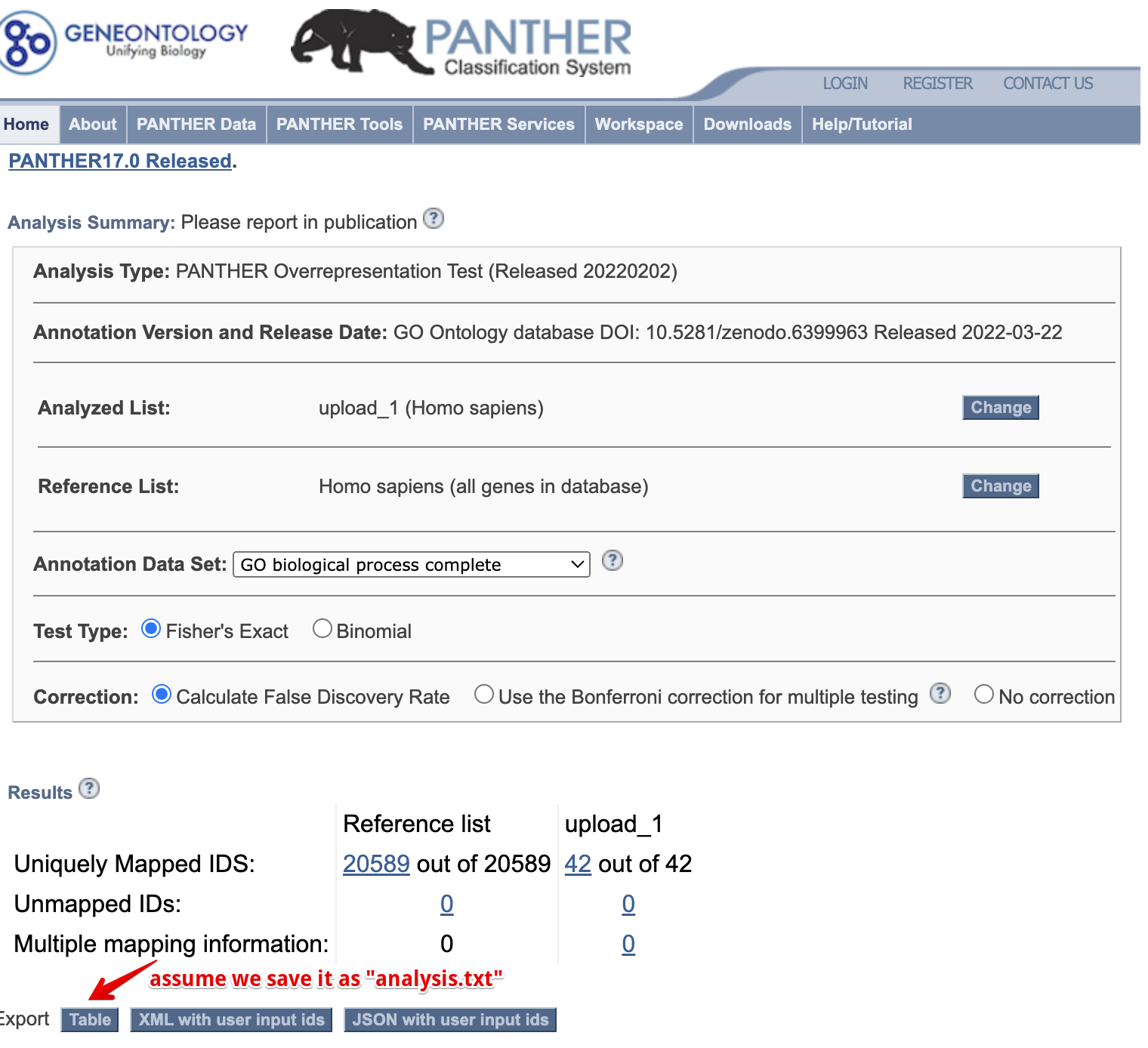
Figure 10.1: Import PANTHER result.
For example, we save the PANTHER result as “analysis.txt” and pass it to importPanther. It will tidy the data and calculate both fold enrichment and rich factor.
panther_res <- importPanther("data/analysis.txt")
head(panther_res, 5)
## ID Description
## 1 GO:0038190 VEGF-activated neuropilin signaling pathway
## 2 GO:1902336 positive regulation of retinal ganglion cell axon guidance
## 3 GO:1902669 positive regulation of axon guidance
## 4 GO:0038189 neuropilin signaling pathway
## 5 GO:0090259 regulation of retinal ganglion cell axon guidance
## GeneRatio BgRatio upload_1 (39) upload_1 (expected)
## 1 0.05128205 9.713925e-05 2 0.00
## 2 0.05128205 1.457089e-04 2 0.01
## 3 0.05128205 1.942785e-04 2 0.01
## 4 0.05128205 1.942785e-04 2 0.01
## 5 0.05128205 2.914177e-04 2 0.01
## upload_1 (over/under) FoldEnrich pvalue qvalue Count RichFactor
## 1 + 527.9231 2.08e-05 0.00289 2 9.713925e-05
## 2 + 351.9487 3.47e-05 0.00429 2 9.713925e-05
## 3 + 263.9615 5.20e-05 0.00558 2 9.713925e-05
## 4 + 263.9615 5.20e-05 0.00555 2 9.713925e-05
## 5 + 175.9744 9.68e-05 0.00904 2 9.713925e-05Then, you can select the terms of interest and utilize the plot functions in Chapter 11.
For example:
plotEnrich(panther_res[c(50,100,350,580,700),],
           plot_type = "bar",
           stats_metric = "qvalue",
           term_metric = "GeneRatio",
           main_text_size = 13,
           legend_text_size = 10
           )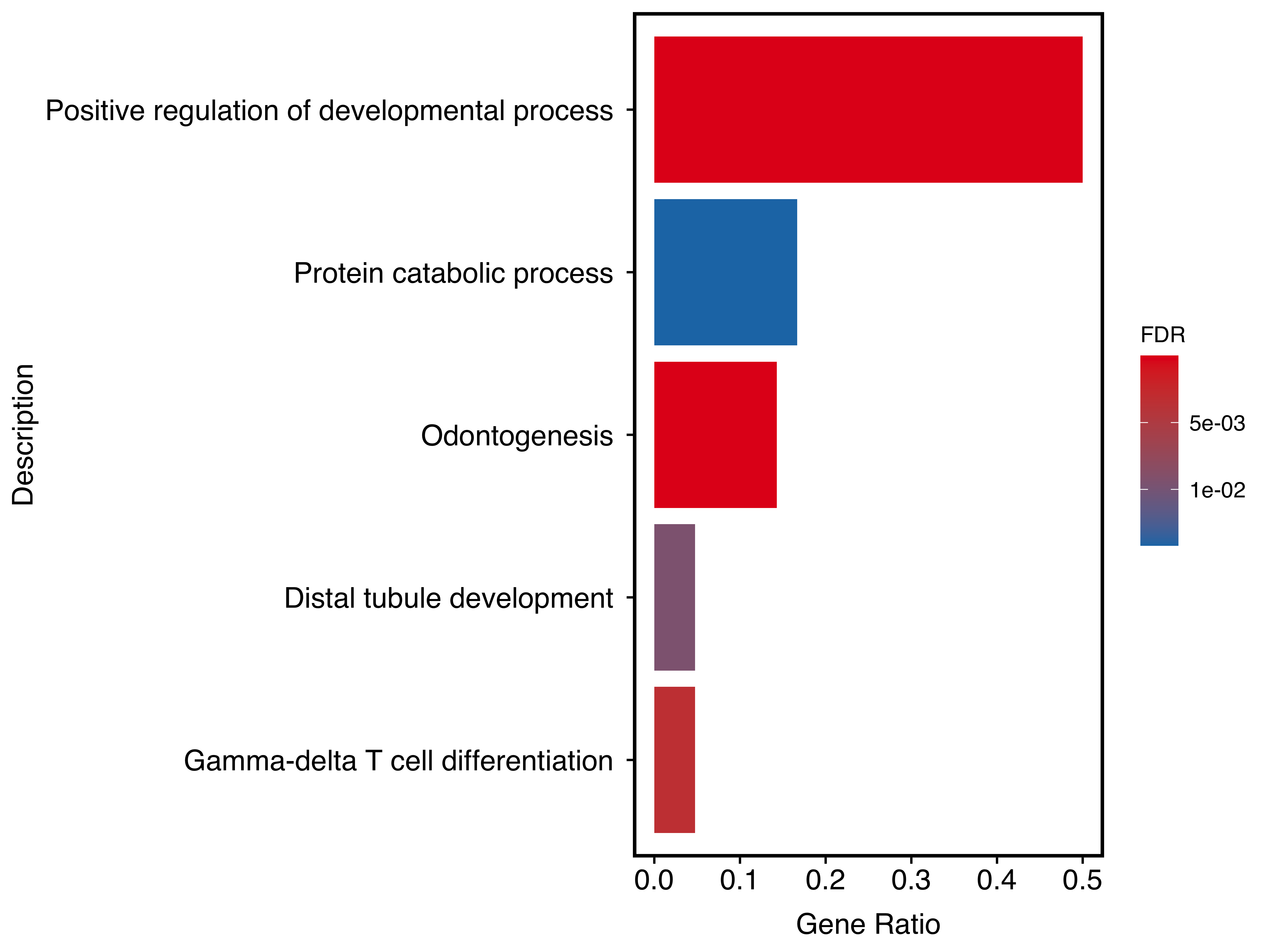
Figure 10.2: Bar plot of PANTHER result.
10.2 Import clusterProfiler object
clusterProfiler is a popular R package for enrichment analysis. However, it requires users to have some programming skills to work with its S4 object, which can be inconvenient for data cleaning and visualization.
Here, genekitr::importCP() can easily import the S4 object along with additional attributes (e.g. FoldEnrich, RichFactor) to help users interact with the data more fluently.
10.2.1 clusterProfiler ORA-GO result
## example data
library(clusterProfiler)
library(org.Hs.eg.db)
data(geneList, package="DOSE")
gene <- names(geneList)[abs(geneList) > 2]

## GO result from clusterProfiler
go <- enrichGO(gene          = gene,
                OrgDb         = org.Hs.eg.db,
                ont           = "BP",
                pAdjustMethod = "BH",
                pvalueCutoff  = 0.01,
                qvalueCutoff  = 0.05)

isS4(go) # return a S4 object
## [1] TRUE
## import
go_easy <- importCP(go, type = "go")
is.data.frame(go_easy)
## [1] TRUE
# keep the same as the original result
identical(as.data.frame(go)[,1], go_easy[,1])
## [1] TRUE
head(go_easy)## hs_BP_ID Description GeneRatio BgRatio
## GO:0140014 GO:0140014 mitotic nuclear division 0.1752577 286/18866
## GO:0000280 GO:0000280 nuclear division 0.1855670 428/18866
## GO:0048285 GO:0048285 organelle fission 0.1907216 476/18866
## GO:0000070 GO:0000070 mitotic sister chromatid segregation 0.1237113 161/18866
## GO:0000819 GO:0000819 sister chromatid segregation 0.1288660 196/18866
## GO:0007059 GO:0007059 chromosome segregation 0.1494845 334/18866
## pvalue p.adjust qvalue
## GO:0140014 2.171838e-26 6.700119e-23 5.710790e-23
## GO:0000280 1.099719e-22 1.696316e-19 1.445841e-19
## GO:0048285 4.058841e-22 4.173841e-19 3.557538e-19
## GO:0000070 3.322345e-21 2.562358e-18 2.184005e-18
## GO:0000819 2.422383e-20 1.494610e-17 1.273918e-17
## GO:0007059 9.308954e-19 4.786354e-16 4.079608e-16
## geneID
## GO:0140014 55143/991/9493/1062/4605/9133/10403/23397/9787/11065/51203/22974/10460/4751/27338/983/4085/81930/81620/332/3832/7272/64151/9212/1111/9319/9055/3833/146909/6790/891/24137/9232/652
## GO:0000280 55143/991/9493/1062/4605/9133/10403/7153/23397/259266/9787/11065/51203/22974/10460/4751/27338/983/4085/81930/81620/332/3832/7272/64151/9212/1111/9319/9055/3833/146909/6790/891/24137/9232/652
## GO:0048285 55143/991/9493/1062/4605/9133/10403/7153/23397/259266/9787/11065/51203/22974/10460/4751/27338/983/4085/81930/81620/332/3832/7272/64151/9212/1111/9319/9055/3833/146909/6790/891/24137/9232/652/4137
## GO:0000070 55143/991/9493/1062/10403/23397/9787/11065/51203/10460/4751/4085/81930/81620/7272/64151/9212/9319/9055/3833/146909/891/24137/9232
## GO:0000819 55143/991/9493/1062/10403/7153/23397/9787/11065/51203/10460/4751/4085/81930/81620/7272/64151/9212/9319/9055/3833/146909/891/24137/9232
## GO:0007059 55143/991/9493/1062/10403/7153/23397/9787/11065/55355/220134/51203/10460/4751/55839/4085/81930/81620/332/7272/64151/9212/9319/9055/3833/146909/891/24137/9232
## geneID_symbol
## GO:0140014 CDCA8/CDC20/KIF23/CENPE/MYBL2/CCNB2/NDC80/NCAPH/DLGAP5/UBE2C/NUSAP1/TPX2/TACC3/NEK2/UBE2S/CDK1/MAD2L1/KIF18A/CDT1/BIRC5/KIF11/TTK/NCAPG/AURKB/CHEK1/TRIP13/PRC1/KIFC1/KIF18B/AURKA/CCNB1/KIF4A/PTTG1/BMP4
## GO:0000280 CDCA8/CDC20/KIF23/CENPE/MYBL2/CCNB2/NDC80/TOP2A/NCAPH/ASPM/DLGAP5/UBE2C/NUSAP1/TPX2/TACC3/NEK2/UBE2S/CDK1/MAD2L1/KIF18A/CDT1/BIRC5/KIF11/TTK/NCAPG/AURKB/CHEK1/TRIP13/PRC1/KIFC1/KIF18B/AURKA/CCNB1/KIF4A/PTTG1/BMP4
## GO:0048285 CDCA8/CDC20/KIF23/CENPE/MYBL2/CCNB2/NDC80/TOP2A/NCAPH/ASPM/DLGAP5/UBE2C/NUSAP1/TPX2/TACC3/NEK2/UBE2S/CDK1/MAD2L1/KIF18A/CDT1/BIRC5/KIF11/TTK/NCAPG/AURKB/CHEK1/TRIP13/PRC1/KIFC1/KIF18B/AURKA/CCNB1/KIF4A/PTTG1/BMP4/MAPT
## GO:0000070 CDCA8/CDC20/KIF23/CENPE/NDC80/NCAPH/DLGAP5/UBE2C/NUSAP1/TACC3/NEK2/MAD2L1/KIF18A/CDT1/TTK/NCAPG/AURKB/TRIP13/PRC1/KIFC1/KIF18B/CCNB1/KIF4A/PTTG1
## GO:0000819 CDCA8/CDC20/KIF23/CENPE/NDC80/TOP2A/NCAPH/DLGAP5/UBE2C/NUSAP1/TACC3/NEK2/MAD2L1/KIF18A/CDT1/TTK/NCAPG/AURKB/TRIP13/PRC1/KIFC1/KIF18B/CCNB1/KIF4A/PTTG1
## GO:0007059 CDCA8/CDC20/KIF23/CENPE/NDC80/TOP2A/NCAPH/DLGAP5/UBE2C/HJURP/SKA1/NUSAP1/TACC3/NEK2/CENPN/MAD2L1/KIF18A/CDT1/BIRC5/TTK/NCAPG/AURKB/TRIP13/PRC1/KIFC1/KIF18B/CCNB1/KIF4A/PTTG1
## Count FoldEnrich RichFactor
## GO:0140014 34 11.560882 0.11888112
## GO:0000280 36 8.179690 0.08411215
## GO:0048285 37 7.559148 0.07773109
## GO:0000070 24 14.496510 0.14906832
## GO:0000819 25 12.404008 0.12755102
## GO:0007059 29 8.443638 0.08682635Then you can select the terms of interest and utilize the plot functions in Chapter 11.
For example:
plotEnrich(tail(go_easy,20),
           plot_type = "genechord",
           show_gene = c("UBE2C", "CDC20", "NDC80"),
           main_text_size = 10,
           legend_text_size = 10
           )
Figure 10.3: Chord plot of clusterProfiler result.
10.2.2 clusterProfiler GSEA result
library(org.Hs.eg.db)
data(geneList, package="DOSE")
## GSEA result from clusterProfiler
kk <- gseGO(geneList     = geneList,
               OrgDb         = org.Hs.eg.db,
               minGSSize    = 400,
               pvalueCutoff = 0.01,
               eps = 0,
               verbose      = FALSE)

## import
kk_easy <- importCP(kk,type = 'gsea')
identical(kk@result[,1], kk_easy$gsea_df[,1])
## [1] TRUEThen you can select the terms of interest and utilize the plot functions in Chapter 12.
For example:
plotGSEA(kk_easy, plot_type = "bar",
         main_text_size = 15)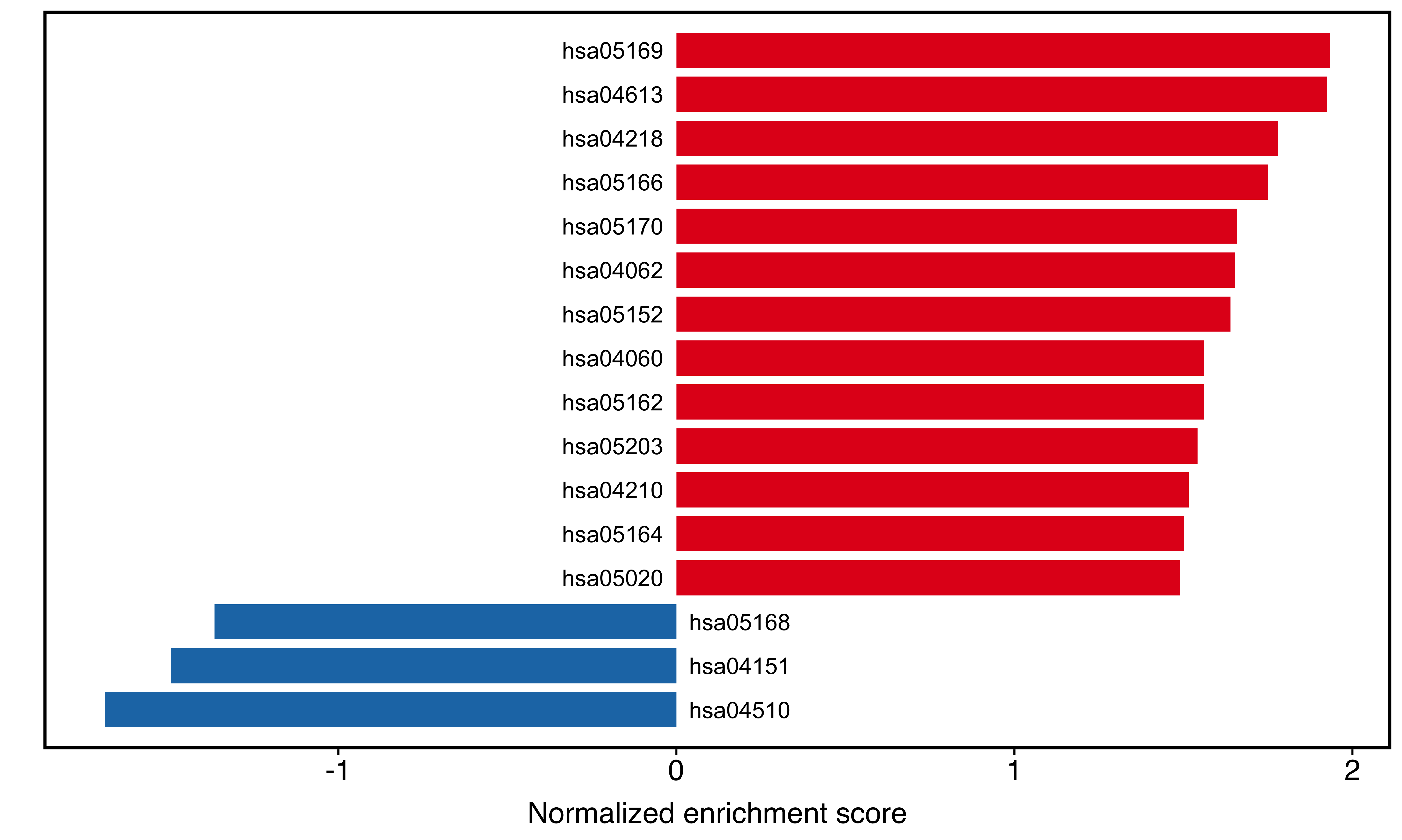
Figure 10.4: Two-side bar plot of clusterProfiler result.
The IDs in the plot are actually from the ID column in the kk_easy result. If you want to add more content, just modify the ID column:
kk_easy$gsea_df$ID <- paste(kk_easy$gsea_df$ID, kk_easy$gsea_df$Description,sep = ": ")
plotGSEA(kk_easy, plot_type = "bar",
         main_text_size = 15)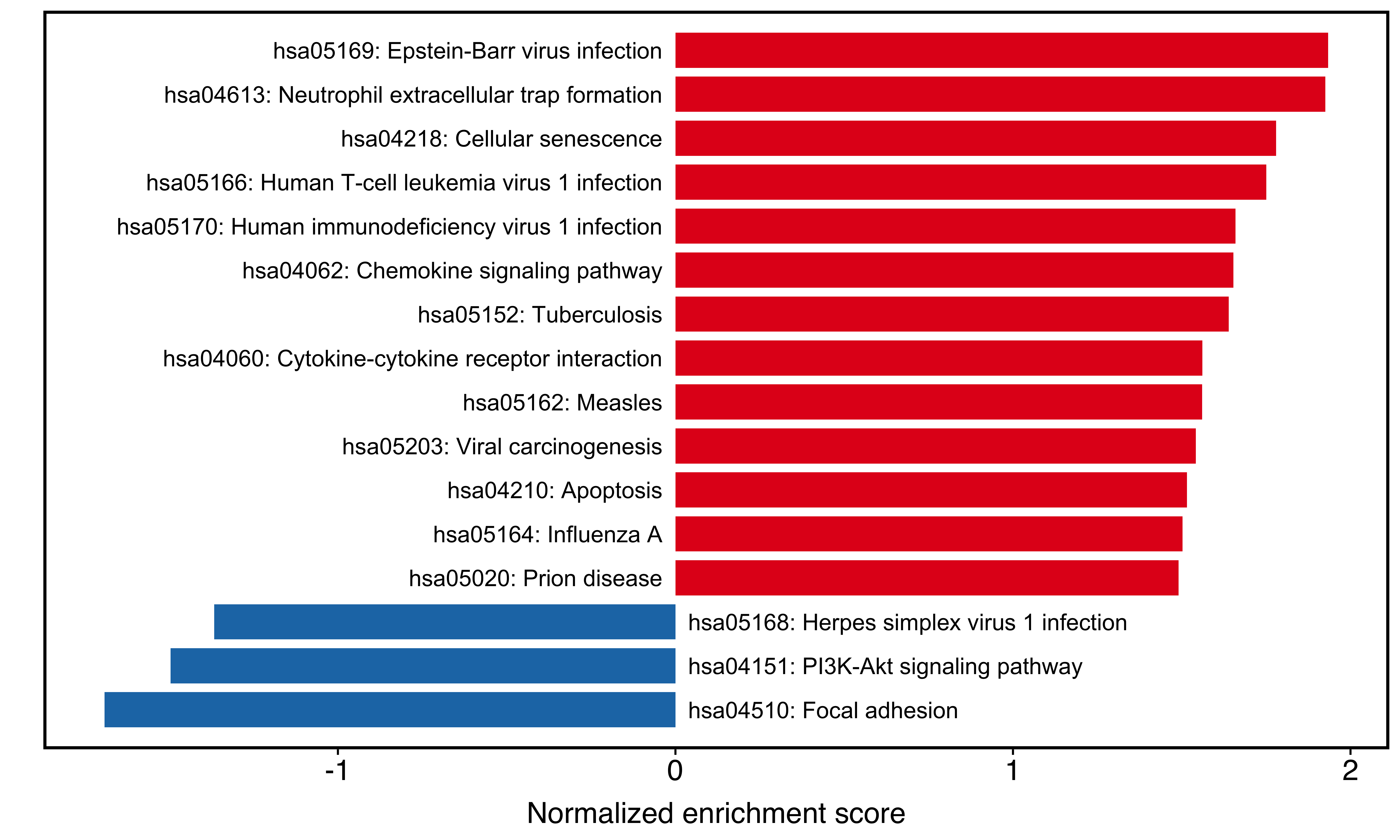
Figure 10.5: Two-side bar plot after modifying labels.
10.2.3 clusterProfiler KEGG/DOSE/WikiPathways… result
clusterProfiler supports many gene sets, including Disease Ontology (DO), WikiPathways and ReactomePA.
Take DO as an example:
library(DOSE)
data(geneList)
gene <- names(geneList)[abs(geneList) > 1.5]

## ORA-DO result from clusterProfiler
do <- enrichDO(gene          = gene,
              ont           = "DO",
              pvalueCutoff  = 0.05,
              pAdjustMethod = "BH",
              universe      = names(geneList),
              minGSSize     = 5,
              maxGSSize     = 500,
              qvalueCutoff  = 0.05)

# import
do_easy <- importCP(do,type = 'other')
identical(as.data.frame(do)[,1], do_easy[,1])
## [1] TRUEThen you can select the terms of interest and utilize the plot functions in Chapter 11.
For example:
plotEnrich(do_easy,
           plot_type = "geneheat",
           fold_change = geneList,
           show_gene = c('S100A9','AGTR1','BIRC5','MMP1','CXCL10'))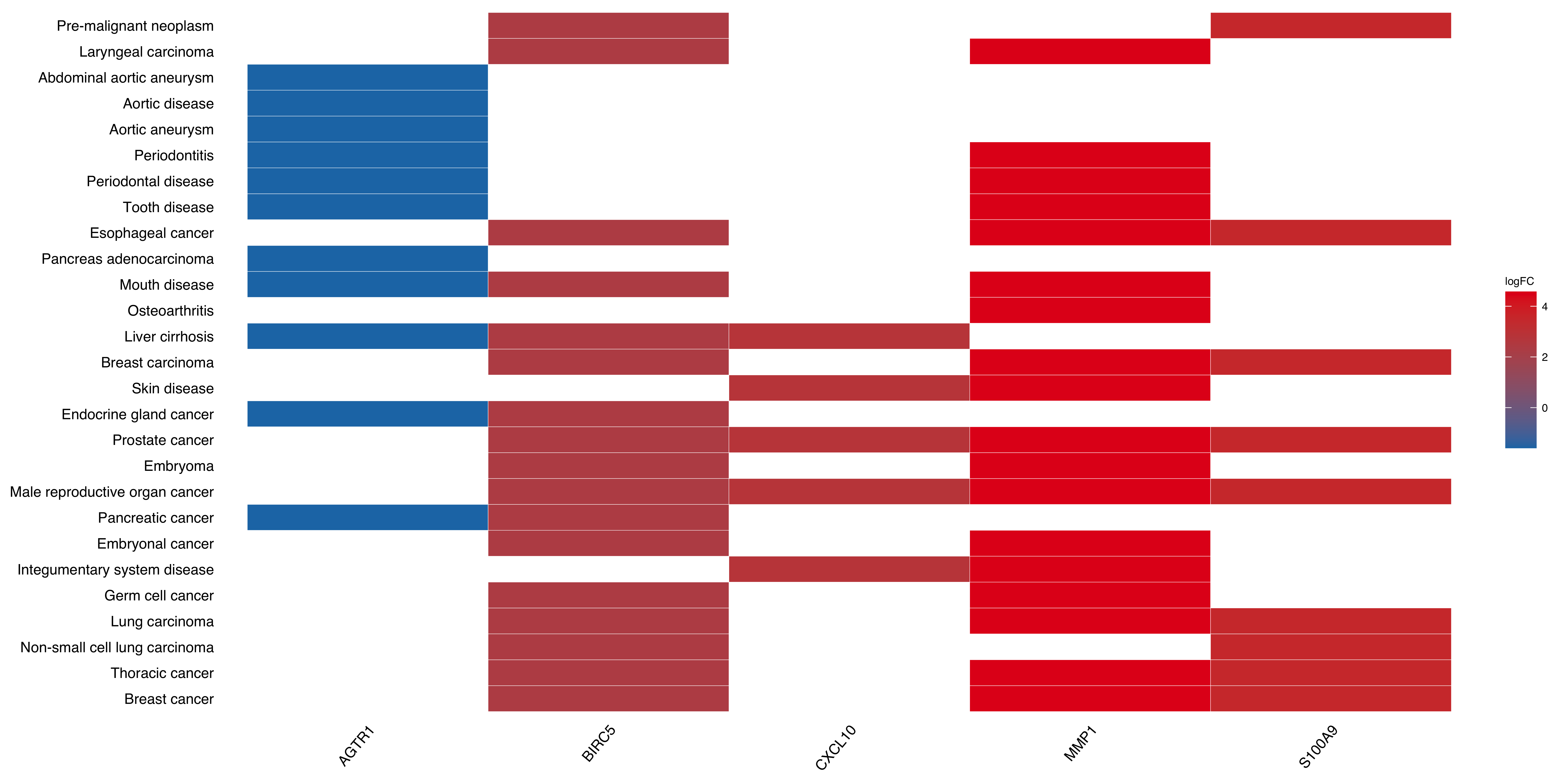
Figure 10.6: Heatmap of clusterProfiler result.